QuickBytes is a series of articles for simple and easy to implement techniques with exponential benefits

The Pivot table is quite a versatile feature and quite popular. This article covers three settings that enhance the user’s experience while using a Pivot Table.
Field List Layout
We get the following layout for the Pivot Table Field List:

It works fine if the list of fields is small. However, I find the following layout more useful:

It offers better visibility of the field lists and convenient to use, especially in small screens.
To enable this, click on the gear icon > Fields Section and Areas Section Side-By-Side

Sort Items in the Field Lists
By default, the sort order of the items in the field lists are according to the data source table:

It becomes a challenge to find any specific field if the list is long. I prefer sorting it in alphabetical order, which makes the finding the field more convenient as it is convenient to find words in alphabetical order:

Click on the gear icon > Sort A to Z

Uncheck GetPivotData
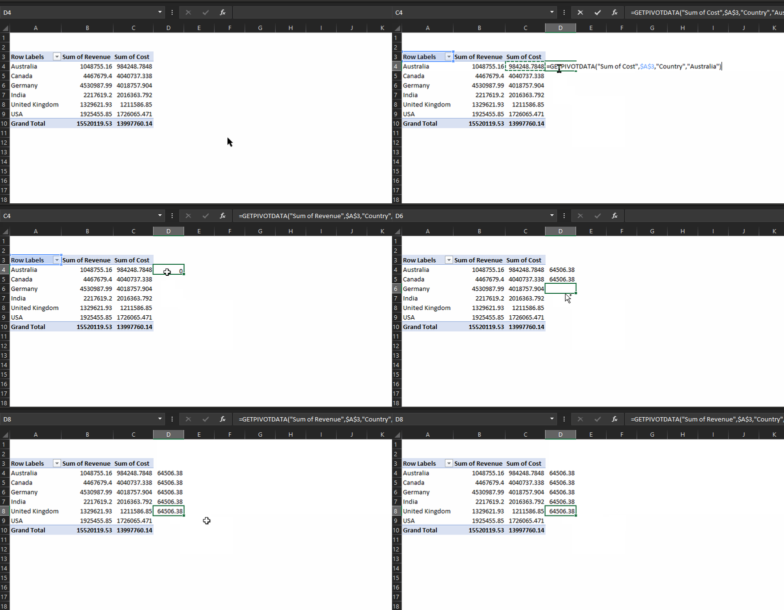
Usually, I prefer to perform some quick calculation next to the Pivot table.
For example, in the pivot table below, I need a column to apply a formula in cell D4 as (B4 – C4)

But instead, I get a rather large formula. It is not dynamic either, when I replicate the formula in all the cells.

We can rectify this by unchecking the option of Generate GetPivotData
PivotTable Analyze > Options > Generate GetPivotData


