Exponential Smoothing forecasts future values by taking the weighted average of previous values. It calculates the weighted average by using a smoothing factor (α).
The exponential smoothing method is adaptive for recent changes in the data points.
Types of Exponential Smoothing:
· Simple Exponential Smoothing: Time series does not contain trend and seasonality.

· Holt’s Exponential Smoothing: Time series data has trend but no seasonality

· Holt Winter’s Exponential Smoothing: When the time series data has both trend and seasonality

Please refer to the article Time Series patterns for more details.
This article explains the Simple Exponential Smoothing.
Simple Exponential Smoothing
Exponential Smoothing uses a weighted average of past time series values as a forecast for future data points

Where

α decides how much smoothing the model is doing
Alternatively, Simple exponential smoothing can also be expressed by:

The new forecast is equal to the previous forecast, plus an adjustment, which is the smoothing constant α times the last forecast error (Actual – Forecast). In other words, we adjust the previous forecast by the fraction of the last forecast error to get the new forecast.
How to select the value of α?
If the variation in the time series data due to random causes (high random variability), a small value of α is preferred. If much of the forecast error is due to random variability, we do not want to overreact and adjust the forecasts too quickly.
For a time-series with low random variability, a forecast error is more likely to represent a real change. Hence, larger values of α provide the advantage of quickly adjusting the forecasts to changes in the time series, thereby allowing the forecasts to react more rapidly to changing conditions.
Industry practice is to set around .20. You may use trial and error method, or Solver to find out the best value of α to improve forecast accuracy.
How to calculate Simple Exponential Smoothing in Excel?
Let us consider the following table:

First, we validate the time series pattern (no trend or seasonality) by plotting a line graph:

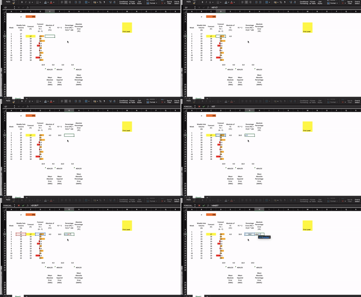
Now, let us apply the formula. To initialize the calculation, we set the exponential smoothing forecast for week 2 equal to the actual value of week 1 and we calculate the forecast accuracy for week 2:

For week 3 forecast, we use the following formula:
= C7+(D7 * C2) // Previous forecast - (Previous forecast error * smoothing constant)
And then apply formulas for calculating forecast accuracy metrics, which we can use to compare different forecasting models.

Please refer to the article for more details: Comparing forecasting models
Plotting the actual vs. forecast:

So, the forecast for week 12 is 18, and the forecast error is 3.5, we can use this to generate the forecast for week 13:
Forecast (w 13) = 18 + 3.5*0.20 = 19
You can use a feature available in Excel called Forecast Sheet, which uses Holt’s Winter Exponential Smoothing method for predictions (suitable for time series with trend and/or seasonality).
